Examples
Reading and plotting Metop ASCAT Surface Soil Moisture CDR (NetCDF)
H SAF provides the following Metop ASCAT Surface Soil Moisture (SSM) Climate Data Record (CDR) products:
H25 - Metop ASCAT SSM CDR2014 : Metop ASCAT Surface Soil Moisture CDR2014 time series 12.5 km sampling
H109 - Metop ASCAT SSM CDR2015 : Metop ASCAT Surface Soil Moisture CDR2015 time series 12.5 km sampling
H111 - Metop ASCAT SSM CDR2016 : Metop ASCAT Surface Soil Moisture CDR2016 time series 12.5 km sampling
The following CDR extensions are also provided by H SAF:
H108 - Metop ASCAT SSM CDR2014-EXT : Metop ASCAT Surface Soil Moisture CDR2014-EXT time series 12.5 km sampling
H110 - Metop ASCAT SSM CDR2015-EXT : Metop ASCAT Surface Soil Moisture CDR2015-EXT time series 12.5 km sampling
H112 - Metop ASCAT SSM CDR2016-EXT : Metop ASCAT Surface Soil Moisture CDR2016-EXT time series 12.5 km sampling
Example H SAF Metop ASCAT SSM DR products
The following example shows how to read and plot H SAF Metop ASCAT SSM data record products using the test data included in the ascat package.
import os
import matplotlib.pyplot as plt
from ascat.h_saf import AscatSsmDataRecord
test_data_path = os.path.join('..', 'tests','ascat_test_data', 'hsaf')
h109_path = os.path.join(test_data_path, 'h109')
h110_path = os.path.join(test_data_path, 'h110')
h111_path = os.path.join(test_data_path, 'h111')
grid_path = os.path.join(test_data_path, 'grid')
static_layer_path = os.path.join(test_data_path, 'static_layer')

h109_dr = AscatSsmDataRecord(h109_path, grid_path, static_layer_path=static_layer_path)
h110_dr = AscatSsmDataRecord(h110_path, grid_path, static_layer_path=static_layer_path)
h111_dr = AscatSsmDataRecord(h111_path, grid_path, static_layer_path=static_layer_path)
A soil moisture time series is read for a specific grid point. The
data attribute contains a pandas.DataFrame object.
gpi = 2501225
h109_ts = h109_dr.read(gpi)
Time series plots
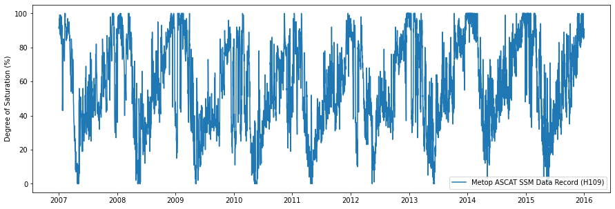
A simple time series plot of surface soil moisture can be created using
matplotlib.
fig, ax = plt.subplots(1, 1, figsize=(15, 5))
ax.plot(h109_ts['sm'], label='Metop ASCAT SSM Data Record (H109)')
ax.set_ylabel('Degree of Saturation (%)')
ax.legend()
<matplotlib.legend.Legend at 0x7fb874034dd8>
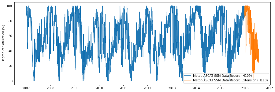
The SSM data record H109 can be extended using H110, representing a consistent continuation of the data set
h110_ts = h110_dr.read(gpi)

fig, ax = plt.subplots(1, 1, figsize=(15, 5))
ax.plot(h109_ts['sm'], label='Metop ASCAT SSM Data Record (H109)')
ax.plot(h110_ts['sm'], label='Metop ASCAT SSM Data Record Extension (H110)')
ax.set_ylabel('Degree of Saturation (%)')
ax.legend()
<matplotlib.legend.Legend at 0x7fb86a725588>
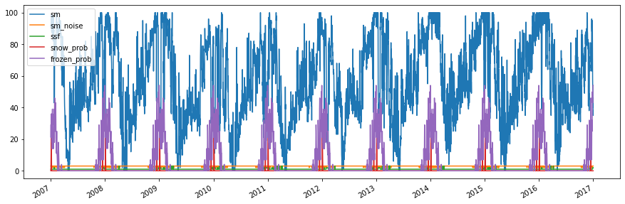
A soil moisture time series can also be plotted using the plot function
provided by the pandas.DataFrame. The following example displays
several variables stored in the time series.
fields = ['sm', 'sm_noise', 'ssf', 'snow_prob', 'frozen_prob']
h111_ts = h111_dr.read(gpi)

fig, ax = plt.subplots(1, 1, figsize=(15, 5))
h111_ts[fields].plot(ax=ax)
ax.legend()
<matplotlib.legend.Legend at 0x7fb86a6840f0>
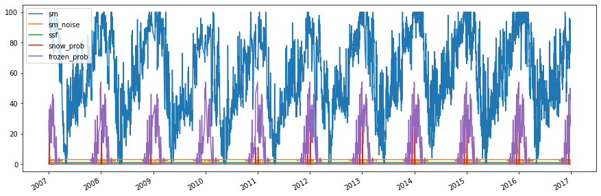
Masking invalid soil moisture measurements
In order to mask invalid/suspicious soil moisture measurements, the confidence flag can be used. It masks soil moisture measurements with a frozen or snow cover probability > 50% and using the Surface State Flag (SSF).
conf_flag_ok = h111_ts['conf_flag'] == 0

fig, ax = plt.subplots(1, 1, figsize=(15, 5))
h111_ts[conf_flag_ok][fields].plot(ax=ax)
ax.legend()
<matplotlib.legend.Legend at 0x7fb86a4afb00>
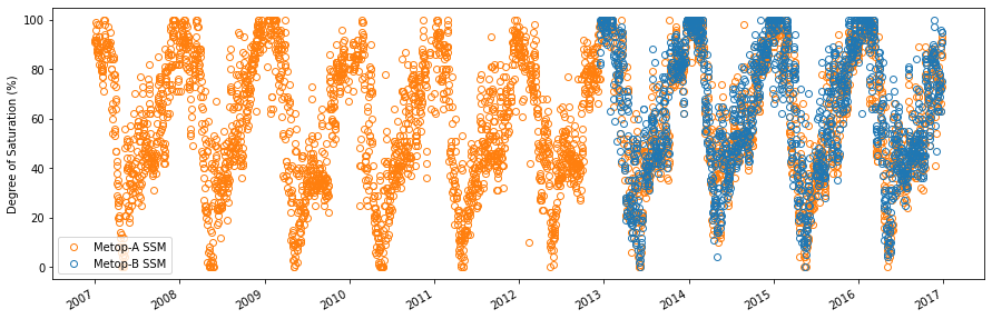
Differentiate between soil moisture from Metop satellites
The sat_id field can be used to differentiate between: Metop-A
(sat_id=3), Metop-B (sat_id=4) and Metop-C (sat_id=5).
metop_a = h111_ts[conf_flag_ok]['sat_id'] == 3
metop_b = h111_ts[conf_flag_ok]['sat_id'] == 4

fig, ax = plt.subplots(1, 1, figsize=(15, 5))
h111_ts[conf_flag_ok]['sm'][metop_a].plot(ax=ax, ls='none', marker='o',
                                          color='C1', fillstyle='none', label='Metop-A SSM')
h111_ts[conf_flag_ok]['sm'][metop_b].plot(ax=ax, ls='none', marker='o',
                                          color='C0', fillstyle='none', label='Metop-B SSM')
ax.set_ylabel('Degree of Saturation (%)')
ax.legend()
<matplotlib.legend.Legend at 0x7fb86a6e2a20>
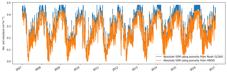
Convert to absolute surface soil moisture
It is possible to convert relative surface soil moisture given in degree
of saturation into absolute soil moisture (\(m^3 m^{-3}\)) using the
absolute_sm keyword during reading. Porosity information provided by
Noah GLDAS and
pre-computed porosity from the Harmonized World Soil Database
(HWSD)
using the formulas of Saxton and Rawls
(2006)
is used to produce volumetric surface soil moisture expressed in
\(m^{3} m^{-3}\).
h111_ts = h111_dr.read(gpi, absolute_sm=True)
conf_flag_ok = h111_ts['conf_flag'] == 0

fig, ax = plt.subplots(1, 1, figsize=(15, 5))
h111_ts[conf_flag_ok]['abs_sm_gldas'].plot(ax=ax, label='Absolute SSM using porosity from Noah GLDAS')
h111_ts[conf_flag_ok]['abs_sm_hwsd'].plot(ax=ax, label='Absolute SSM using porosity from HWSD')
ax.set_ylabel('Vol. soil moisture ($m^3 m^{-3}$)')
ax.legend()
<matplotlib.legend.Legend at 0x7fb86a39be10>
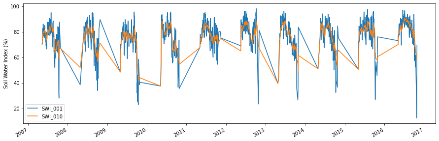
Reading and plotting CGLS SWI_TS data (NetCDF)
This example script reads the SWI_TS product of the Copernicus Global Land Service.
If the standard file names assumed by the script have changed this can be
specified during initialization of the SWI_TS object. Please see the
documentation of ascat.cgls.SWI_TS.
Example CGLS SWI time series
import os
from ascat.cgls import SWI_TS
import matplotlib.pyplot as plt
%matplotlib inline
By default we should have the grid file from the SWI-STATIC collection and the unzipped SWI-TS products in one folder like so:
ls ../tests/ascat_test_data/cglops/swi_ts
c_gls_SWI-STATIC-DGG_201501010000_GLOBE_ASCAT_V3.0.1.nc
c_gls_SWI-TS_201612310000_C0375_ASCAT_V3.0.1.nc
data_path = os.path.join('..', 'tests', 'ascat_test_data', 'cglops', 'swi_ts')
rd = SWI_TS(data_path)
data = rd.read_ts(3002621)
print(data)
                     SWI_001  SWI_005  SWI_010  SWI_015  SWI_020  SWI_040  2007-05-10 12:00:00     70.0     71.0     71.0     71.0     71.0     71.0
2007-05-14 12:00:00     71.5     71.5     71.5     71.5     71.5     71.5
2007-05-15 12:00:00     82.0     78.0     77.0     76.5     76.5     76.0
2007-05-16 12:00:00     82.5     79.0     78.0     77.5     77.0     77.0
2007-05-17 12:00:00     77.5     77.5     77.0     76.5     76.5     76.0
...                      ...      ...      ...      ...      ...      ...
2016-10-14 12:00:00     55.0     60.0     65.5     69.0     71.0     76.5
2016-10-15 12:00:00     56.5     59.0     64.5     68.0     70.5     75.5
2016-10-16 12:00:00     61.5     60.0     64.5     67.5     70.0     75.5
2016-10-26 12:00:00     12.5     42.5     59.0     64.5     68.0     74.5
2016-10-28 12:00:00     69.5     54.0     60.0     64.5     67.5     74.0

                     SWI_060  SWI_100  SSF
2007-05-10 12:00:00      NaN      NaN  1.0
2007-05-14 12:00:00     71.5      NaN  1.0
2007-05-15 12:00:00     76.0     76.0  1.0
2007-05-16 12:00:00     77.0     76.5  1.0
2007-05-17 12:00:00     76.0     76.0  1.0
...                      ...      ...  ...
2016-10-14 12:00:00     78.5     80.0  1.0
2016-10-15 12:00:00     78.0     80.0  1.0
2016-10-16 12:00:00     78.0     79.5  1.0
2016-10-26 12:00:00     77.0     79.0  1.0
2016-10-28 12:00:00     76.5     79.0  1.0

[1603 rows x 9 columns]
Since the returned value is a pandas.DataFrame we can plot the data easily.
fig, ax = plt.subplots(1, 1, figsize=(15, 5))
data[['SWI_001', 'SWI_010']].plot(ax=ax)
ax.set_ylabel('Soil Water Index (%)')
plt.show()
Reading and plotting H SAF NRT Surface Soil Moisture products (BUFR)
H SAF provides the following NRT surface soil moisture products:
(H07 - SM OBS 1 : Large scale surface soil moisture by radar scatterometer in BUFR format over Europe) - discontinued
H08 - SSM ASCAT NRT DIS : Disaggregated Metop ASCAT NRT Surface Soil Moisture at 1 km
H14 - SM DAS 2 : Profile index in the roots region by scatterometer data assimilation in GRIB format
H101 - SSM ASCAT-A NRT O12.5 : Metop-A ASCAT NRT Surface Soil Moisture 12.5km sampling
H102 - SSM ASCAT-A NRT O25 : Metop-A ASCAT NRT Surface Soil Moisture 25 km sampling
H16 - SSM ASCAT-B NRT O12.5 : Metop-B ASCAT NRT Surface Soil Moisture 12.5 km sampling
H103 - SSM ASCAT-B NRT O25 : Metop-B ASCAT NRT Surface Soil Moisture 25 km sampling
The products H101, H102, H16, H103 come in BUFR format and can be read by the same reader. So examples for the H16 product are equally valid for the other products.
The product H07 is discontinued and replaced by Metop-A (H101, H102) and Metop-B (H103, H16), both available in two different resolutions.
The following example will show how to read and plot each of them.
Example H SAF SM NRT products
In this Example we will read and plot images of the H SAF NRT products H08, H14 and H16 using the test images included in the ascat package.
import os
from datetime import datetime
import numpy as np
import cartopy
import matplotlib.pyplot as plt
from pytesmo.grid.resample import resample_to_grid
%matplotlib inline

from ascat.h_saf import H08BufrFileList
from ascat.h_saf import H14GribFileList
from ascat.h_saf import AscatNrtBufrFileList
/home/shahn/conda/ascat_conda/envs/ascat_env/lib/python3.6/site-packages/pyresample/bilinear/__init__.py:49: UserWarning: XArray and/or zarr not found, XArrayBilinearResampler won't be available.
  warnings.warn("XArray and/or zarr not found, XArrayBilinearResampler won't be available.")
/home/shahn/conda/ascat_conda/envs/ascat_env/lib/python3.6/site-packages/pytesmo/grid/resample.py:30: UserWarning: resampling functions have moved to the repurpose package and will beremoved from pytesmo soon!
  warn("resampling functions have moved to the repurpose package and will be"
test_data_path = os.path.join('..', 'tests','ascat_test_data', 'hsaf')
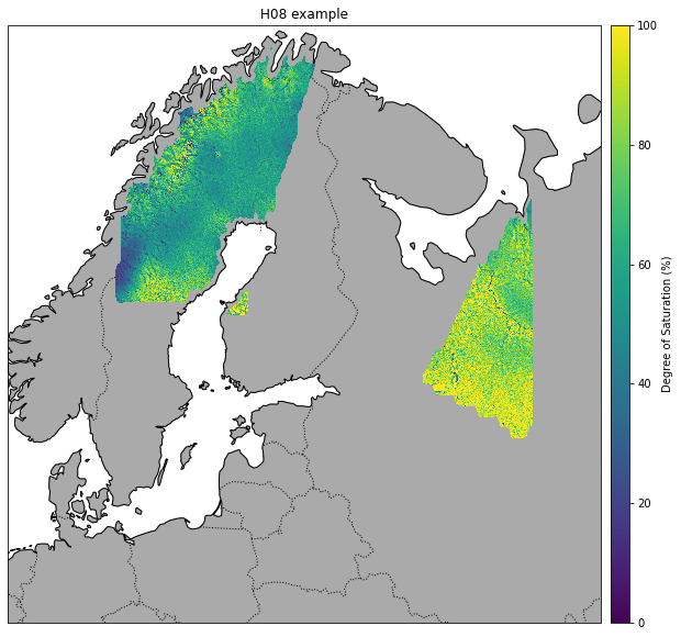
Disaggregated ASCAT SSM NRT (H08)
H08 data has a much higher resolution and comes on a 0.00416 degree grid. The sample data included in the ascat package was observed on the same time as the included H16 product.
h08_path = os.path.join(test_data_path, 'h08')
h08_nrt = H08BufrFileList(h08_path)
h08_data = h08_nrt.read(datetime(2010, 5, 1, 8, 33, 1))
h08_data
{'ssm': array([[1.69999998e+38, 1.69999998e+38, 1.69999998e+38, ...,
         1.69999998e+38, 1.69999998e+38, 1.69999998e+38],
        [1.69999998e+38, 1.69999998e+38, 1.69999998e+38, ...,
         1.69999998e+38, 1.69999998e+38, 1.69999998e+38],
        [1.69999998e+38, 1.69999998e+38, 1.69999998e+38, ...,
         1.69999998e+38, 1.69999998e+38, 1.69999998e+38],
        ...,
        [1.69999998e+38, 1.69999998e+38, 1.69999998e+38, ...,
         1.69999998e+38, 1.69999998e+38, 1.69999998e+38],
        [1.69999998e+38, 1.69999998e+38, 1.69999998e+38, ...,
         1.69999998e+38, 1.69999998e+38, 1.69999998e+38],
        [1.69999998e+38, 1.69999998e+38, 1.69999998e+38, ...,
         1.69999998e+38, 1.69999998e+38, 1.69999998e+38]]),
 'ssm_noise': array([[1.69999998e+38, 1.69999998e+38, 1.69999998e+38, ...,
         1.69999998e+38, 1.69999998e+38, 1.69999998e+38],
        [1.69999998e+38, 1.69999998e+38, 1.69999998e+38, ...,
         1.69999998e+38, 1.69999998e+38, 1.69999998e+38],
        [1.69999998e+38, 1.69999998e+38, 1.69999998e+38, ...,
         1.69999998e+38, 1.69999998e+38, 1.69999998e+38],
        ...,
        [1.69999998e+38, 1.69999998e+38, 1.69999998e+38, ...,
         1.69999998e+38, 1.69999998e+38, 1.69999998e+38],
        [1.69999998e+38, 1.69999998e+38, 1.69999998e+38, ...,
         1.69999998e+38, 1.69999998e+38, 1.69999998e+38],
        [1.69999998e+38, 1.69999998e+38, 1.69999998e+38, ...,
         1.69999998e+38, 1.69999998e+38, 1.69999998e+38]]),
 'proc_flag': array([[1.69999998e+38, 1.69999998e+38, 1.69999998e+38, ...,
         1.69999998e+38, 1.69999998e+38, 1.69999998e+38],
        [1.69999998e+38, 1.69999998e+38, 1.69999998e+38, ...,
         1.69999998e+38, 1.69999998e+38, 1.69999998e+38],
        [1.69999998e+38, 1.69999998e+38, 1.69999998e+38, ...,
         1.69999998e+38, 1.69999998e+38, 1.69999998e+38],
        ...,
        [1.69999998e+38, 1.69999998e+38, 1.69999998e+38, ...,
         1.69999998e+38, 1.69999998e+38, 1.69999998e+38],
        [1.69999998e+38, 1.69999998e+38, 1.69999998e+38, ...,
         1.69999998e+38, 1.69999998e+38, 1.69999998e+38],
        [1.69999998e+38, 1.69999998e+38, 1.69999998e+38, ...,
         1.69999998e+38, 1.69999998e+38, 1.69999998e+38]]),
 'corr_flag': array([[0., 0., 0., ..., 0., 0., 0.],
        [0., 0., 0., ..., 0., 0., 0.],
        [0., 0., 0., ..., 0., 0., 0.],
        ...,
        [0., 0., 0., ..., 0., 0., 0.],
        [0., 0., 0., ..., 0., 0., 0.],
        [0., 0., 0., ..., 0., 0., 0.]]),
 'lon': array([[13.00208, 13.00625, 13.01042, ..., 44.98958, 44.99375, 44.99792],
        [13.00208, 13.00625, 13.01042, ..., 44.98958, 44.99375, 44.99792],
        [13.00208, 13.00625, 13.01042, ..., 44.98958, 44.99375, 44.99792],
        ...,
        [13.00208, 13.00625, 13.01042, ..., 44.98958, 44.99375, 44.99792],
        [13.00208, 13.00625, 13.01042, ..., 44.98958, 44.99375, 44.99792],
        [13.00208, 13.00625, 13.01042, ..., 44.98958, 44.99375, 44.99792]]),
 'lat': array([[70.99792   , 70.99792   , 70.99792   , ..., 70.99792   ,
         70.99792   , 70.99792   ],
        [70.99375333, 70.99375333, 70.99375333, ..., 70.99375333,
         70.99375333, 70.99375333],
        [70.98958666, 70.98958666, 70.98958666, ..., 70.98958666,
         70.98958666, 70.98958666],
        ...,
        [58.01041334, 58.01041334, 58.01041334, ..., 58.01041334,
         58.01041334, 58.01041334],
        [58.00624667, 58.00624667, 58.00624667, ..., 58.00624667,
         58.00624667, 58.00624667],
        [58.00208   , 58.00208   , 58.00208   , ..., 58.00208   ,
         58.00208   , 58.00208   ]])}
plot_crs = cartopy.crs.Mercator()
data_crs = cartopy.crs.PlateCarree()

fig = plt.figure(figsize=(12, 10))
ax = fig.add_subplot(1, 1, 1, projection=plot_crs)
ax.set_title('H08 example')

ax.add_feature(cartopy.feature.COASTLINE, linestyle='-')
ax.add_feature(cartopy.feature.BORDERS, linestyle=':')
ax.add_feature(cartopy.feature.LAND, facecolor='#aaaaaa')
ax.set_extent([5, 50, 50, 70])

ssm = np.ma.masked_greater(np.flipud(h08_data['ssm']), 100)
sc = ax.pcolormesh(h08_data['lon'], np.flipud(h08_data['lat']), ssm, zorder=3,
                   transform=data_crs, vmin=0, vmax=100)

cax = fig.add_axes([ax.get_position().x1+0.01, ax.get_position().y0,
                    0.02, ax.get_position().height])

cbar = fig.colorbar(sc, ax=ax, cax=cax)
cbar.set_label('Degree of Saturation (%)')
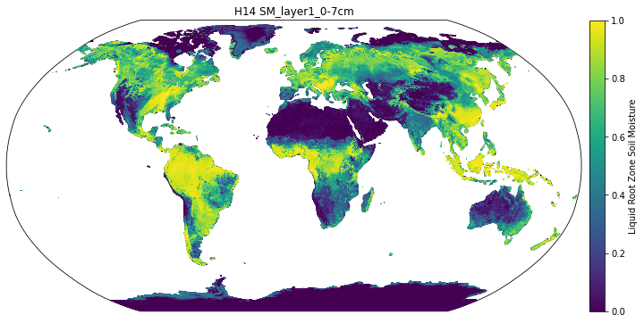
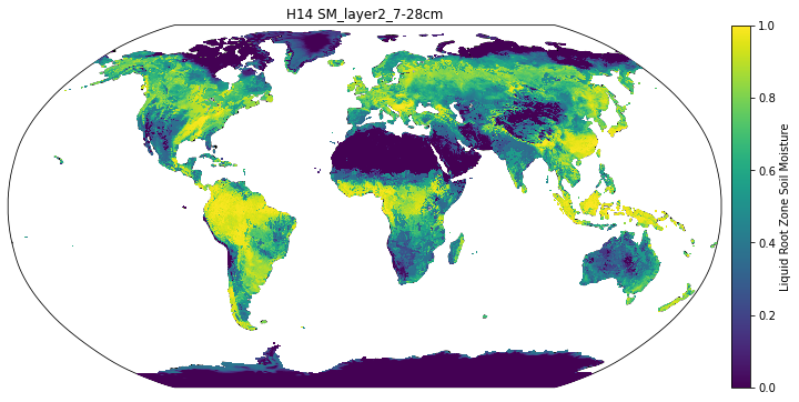
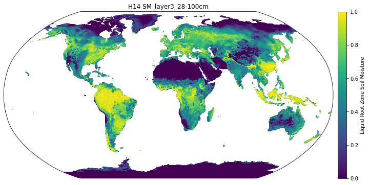
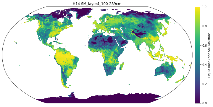
SM-DAS-2 (H14)
The SM-DAS-2 (H14) product is a global product on a reduced gaussian grid with a resolution of approx. 25km.
h14_path = os.path.join(test_data_path, 'h14')
h14_nrt = H14GribFileList(h14_path)
h14_data = h14_nrt.read(datetime(2014, 5, 15))

# the data is a dictionary, each dictionary key contains the array of one variable
print("The following variables are in this image", h14_data.keys())
print(h14_data['SM_layer1_0-7cm'].shape)
print(h14_data['lon'].shape, h14_data['lat'].shape)
The following variables are in this image dict_keys(['SM_layer1_0-7cm', 'lat', 'lon', 'SM_layer2_7-28cm', 'SM_layer3_28-100cm', 'SM_layer4_100-289cm'])
(800, 1600)
(800, 1600) (800, 1600)
Let’s plot all layers in the H14 product
plot_crs = cartopy.crs.Robinson()
data_crs = cartopy.crs.PlateCarree()

layers = ['SM_layer1_0-7cm', 'SM_layer2_7-28cm',
          'SM_layer3_28-100cm', 'SM_layer4_100-289cm']

for layer in layers:
    fig = plt.figure(figsize=(12, 6))
    ax = fig.add_subplot(1, 1, 1, projection=plot_crs)
    ax.set_title('H14 {:}'.format(layer))

    ax.add_feature(cartopy.feature.COASTLINE, linestyle='-')
    ax.add_feature(cartopy.feature.BORDERS, linestyle=':')
    ax.add_feature(cartopy.feature.LAND, facecolor='#aaaaaa')

    sc = ax.pcolormesh(h14_data['lon'], h14_data['lat'], h14_data[layer], zorder=3,
                       transform=data_crs)

    cax = fig.add_axes([ax.get_position().x1+0.01, ax.get_position().y0,
                    0.02, ax.get_position().height])

    cbar = fig.colorbar(sc, ax=ax, cax=cax)
    cbar.set_label('Liquid Root Zone Soil Moisture')
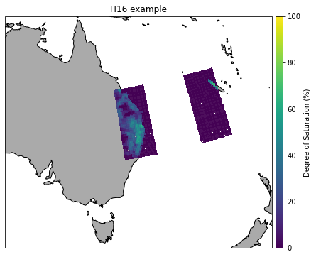
ASCAT SSM NRT (H16, H101, H102, H103)
The products H16, H101, H102, H103 come in the same BUFR format and the default filenames are slightly different.
h16_path = os.path.join(test_data_path, 'h16')
h16_nrt = AscatNrtBufrFileList(h16_path)
h16_data = h16_nrt.read(datetime(2017, 2, 20, 11, 15, 0))

print(h16_data['sm'].shape, h16_data['lon'].shape, h16_data['lat'].shape)
(2016,) (2016,) (2016,)
plot_crs = cartopy.crs.Mercator()
data_crs = cartopy.crs.PlateCarree()

fig = plt.figure(figsize=(7, 6))
ax = fig.add_subplot(1, 1, 1, projection=plot_crs)
ax.set_title('H16 example')

ax.add_feature(cartopy.feature.COASTLINE, linestyle='-')
ax.add_feature(cartopy.feature.BORDERS, linestyle=':')
ax.add_feature(cartopy.feature.LAND, facecolor='#aaaaaa')
ax.set_extent([130, 175, -10, -42])

sc = ax.scatter(h16_data['lon'], h16_data['lat'],
                c=h16_data['sm'], zorder=3, marker='s', s=2,
                transform=data_crs, vmin=0, vmax=100)

cax = fig.add_axes([ax.get_position().x1+0.01, ax.get_position().y0,
                    0.02, ax.get_position().height])
cbar = fig.colorbar(sc, ax=ax, cax=cax)
cbar.set_label('Degree of Saturation (%)')
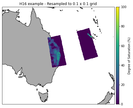
Or resample orbit geometry to a regular 0.1 deg x 0.1 deg grid for plotting
# lets resample to a 0.1 degree grid
# define the grid points in latitude and logitude
lats_dim = np.arange(-80, 80, 0.1)
lons_dim = np.arange(-160, 170, 0.1)

# make 2d grid out the 1D grid spacings
lons_grid, lats_grid = np.meshgrid(lons_dim, lats_dim)

resampled_data = resample_to_grid({'sm': h16_data['sm']}, h16_data['lon'],
                                  h16_data['lat'], lons_grid, lats_grid)

fig = plt.figure(figsize=(7, 6))
ax = fig.add_subplot(1, 1, 1, projection=plot_crs)
ax.set_title('H16 example - Resampled to 0.1 x 0.1 grid')

ax.add_feature(cartopy.feature.COASTLINE, linestyle='-')
ax.add_feature(cartopy.feature.BORDERS, linestyle=':')
ax.add_feature(cartopy.feature.LAND, facecolor='#aaaaaa')
ax.set_extent([130, 175, -10, -42])

sc = ax.pcolormesh(lons_grid, lats_grid, resampled_data['sm'], zorder=3,
                   vmin=0, vmax=100, transform=data_crs)

cax = fig.add_axes([ax.get_position().x1+0.01, ax.get_position().y0,
                    0.02, ax.get_position().height])
cbar = fig.colorbar(sc, ax=ax, cax=cax)
cbar.set_label('Degree of Saturation (%)')
Reading and plotting TU Wien Metop ASCAT Surface Soil Moisture (Binary)
This example program reads and plots Metop ASCAT SSM and SWI data with different masking options. The readers are only provided for the sake of completeness, because the data sets are outdated and superseded by the H SAF Surface Soil Moisture Climate Data Records (e.g. H109, H111). The SWI data sets are replaced by the CGLS SWI product.
Reading and plotting TU Wien Metop ASCAT Vegetation Optical Depth (VOD)
This example program reads and plots Metop ASCAT VOD data.
Reading and plotting lvl1b and lvl2 ASCAT data in generic manner
This example script uses the generic lvl1b and lvl2 reader to get an generic Image.